](https://lastfm.freetls.fastly.net/i/u/770x0/63dce6a777fc491b8c317542037bd15d.webp#63dce6a777fc491b8c317542037bd15d)
Anthony Fantano (@theneedledrop, a.k.a Melon) has been reviewing albums on his YouTube channel for more than one decade. I’ve been enjoying his work and discovering some great music since 2014.
Recently, I was wondering if I could fit a classification model to predict if an album would get a high score from Fantano. Besides, I wanted to understand what features drive his scoring. Surprisingly, I found that danceability isn’t a feature that Melon appreciates.
Using Python and R, I got the audio features of the albums from Spotify using spotipy, cleaned the data in R, fitted and evaluated a predictive model with Scikit-Learn. The whole process is described in this post.
Getting the data
I grabbed data from the Needle Drop reviews and from the albums’ audio features from Spotify API. First, let’s load the packages in R.
#data cleaning and reading
library(tidyverse)
library(lubridate)
library(googlesheets4)
library(reticulate)
use_condaenv("py3.8", required = TRUE)

#dataviz
library(reactable)
library(hrbrthemes)
library(glue)
library(ggtext)
library(ggdist)
library(gghalves)
library(patchwork)
Reviews
Part of the dataset containing the relation of reviews and its scores came from Jared Arcilla’s Kaggle dataset and by one Reddit user (unfortunately, the post was deleted), and later completed by me. The last video in the database is Palais d’Argile by Feu! Chatterton (posted on 2021-03-25). I searched album and artist URI from Spotify using spotipy. The relation of album URI, album title, artist name, artist URI, and review features (date, type, score, and link) were stored on Google Sheets.
gs4_deauth() #the google sheet is public

reviews <-
        read_sheet("https://docs.google.com/spreadsheets/d/1sei8XeqjjznXVOiBpmVWpcB366sM1MBUL5QYV7qxpzs/edit?usp=sharing", col_types = "ccccccDcdcc")
A total of 2350 album reviews were collected. The following 77 albums were not found on Spotify (3% of the reviews).
reviews %>%
        filter(is.na(album_uri)) %>%
        select(title, artist, review_date, score, word_score, link) %>%
        reactable(
                columns = list(
                        title = colDef(name = "Title"),
                        artist = colDef(name = "Artist"),
                        review_date = colDef(name = "Review date"),
                        score = colDef(name = "Score"),
                        word_score = colDef(name = "Word score/observation"),
                        link = colDef(name = "Review link")
                ),
                highlight = TRUE, bordered = TRUE)
Audio features
Later, I pulled the albums’ audio features in Python with spotipy. The code can be accessed here. The following features were gathered, whose description can be found on Spotify Web API documentation:
explicity: “whether or not the track has explicit lyrics (true= yes it does;false= no it does not OR unknown).”acousticness: “a confidence measure from 0.0 to 1.0 of whether the track is acoustic. 1.0 represents high confidence the track is acoustic”danceability: “danceability describes how suitable a track is for dancing based on a combination of musical elements including tempo, rhythm stability, beat strength, and overall regularity. A value of 0.0 is least danceable and 1.0 is most danceable”. Charlie Thompson made a great analysis of the danceability of Thom York’s music projects over time (Radiohead, solo albums, and Atoms for Peace)track_duration: “the duration of the track in milliseconds”energy: “energy is a measure from 0.0 to 1.0 and represents a perceptual measure of intensity and activity. Typically, energetic tracks feel fast, loud, and noisy. For example, death metal has high energy, while a Bach prelude scores low on the scale. Perceptual features contributing to this attribute include dynamic range, perceived loudness, timbre, onset rate, and general entropy”instrumentalness: “predicts whether a track contains no vocals. ‘Ooh’ and ‘aah’ sounds are treated as instrumental in this context. Rap or spoken word tracks are clearly ‘vocal’. The closer the instrumentalness value is to 1.0, the greater likelihood the track contains no vocal content. Values above 0.5 are intended to represent instrumental tracks, but confidence is higher as the value approaches 1.0.”liveness: “detects the presence of an audience in the recording. Higher liveness values represent an increased probability that the track was performed live. A value above 0.8 provides strong likelihood that the track is live”loudness: “the overall loudness of a track in decibels (dB). Loudness values are averaged across the entire track and are useful for comparing relative loudness of tracks. Loudness is the quality of a sound that is the primary psychological correlate of physical strength (amplitude). Values typical range between -60 and 0 db.”speechiness: “speechiness detects the presence of spoken words in a track. The more exclusively speech-like the recording (e.g. talk show, audio book, poetry), the closer to 1.0 the attribute value. Values above 0.66 describe tracks that are probably made entirely of spoken words. Values between 0.33 and 0.66 describe tracks that may contain both music and speech, either in sections or layered, including such cases as rap music. Values below 0.33 most likely represent music and other non-speech-like tracks”tempo: “the overall estimated tempo of a track in beats per minute (BPM).”valence: “a measure from 0.0 to 1.0 describing the musical positiveness conveyed by a track. Tracks with high valence sound more positive (e.g. happy, cheerful, euphoric), while tracks with low valence sound more negative (e.g. sad, depressed, angry).”
I also got the album’s popularity (album_popularity, a value between 0 and 100, with 100 being the most popular) and the list of genres associated with the artist (artist_genres). The gathered data were stored on the spotify_songs.csv file (available on GitHub).
songs <- read.csv("input/spotify_songs.csv")Joining all together
Later, I joined the songs data with the reviews data, extracted the artist genres (1 genre per column). The mean and the standard deviation of each song’s audio feature were summarised by album. Also, I calculated the “Sonic Anger Index” of each album based on its mean energy and valence, following the approach by Even Oppenheimer to find the angriest Death Grips song.
reviews_songs <- reviews %>%
        left_join(songs, by = c("album_id", "album_uri")) %>%
  #removing the type of record (album, ep, ...), the album genres (it is empty) and track numbers from data
  select(-review_type, -album_type, -album_genres, -track_number) %>%
  #extracting one genre per column
  mutate(genre = gsub(pattern = "\\[", replacement = "", artist_genres),
               genre = gsub(pattern = "\\]", replacement = "", genre),
               genre = gsub(pattern = "\\'", replacement = "", genre),
               genre = str_split(genre, pattern = ",")) %>%
        unnest_wider(genre) %>%
        rename(genre_01 = ...1,
               genre_02 = ...2,
               genre_03 = ...3,
               genre_04 = ...4,
               genre_05 = ...5,
               song_name = name) %>%
        mutate_at(c("genre_01", "genre_02", "genre_03", "genre_04", "genre_05"),
                  str_trim) %>%
        mutate_at(c("genre_01", "genre_02", "genre_03", "genre_04", "genre_05"),
                  ~str_replace(., "^$", NA_character_)) %>%
        mutate_at(c("genre_01", "genre_02", "genre_03", "genre_04", "genre_05"),
                  ~str_replace(., "\"", NA_character_)) %>%
        select(album_id:genre_05, -artist_genres, -album)

#extract the mean and std. dev. of the songs features by album
songs_features_by_album <-
  reviews_songs %>%
    group_by(album_id) %>%
        summarise(
                album_length = sum(track_duration_ms),
                mean_track_duration = mean(track_duration_ms, na.rm = TRUE),
                sd_track_duration = sd(track_duration_ms, na.rm = TRUE),
                mean_expl = mean(track_explicity, na.rm = TRUE),
                mean_acousticness = mean(acousticness, na.rm = TRUE),
                sd_acousticness = sd(acousticness, na.rm = TRUE),
                mean_danceability = mean(danceability, na.rm = TRUE),
                sd_danceability = sd(danceability, na.rm = TRUE),
                mean_energy = mean(energy, na.rm = TRUE),
                sd_energy = sd(energy, na.rm = TRUE),
                mean_instrumentalness = mean(instrumentalness, na.rm = TRUE),
                sd_instrumentalness = sd(instrumentalness, na.rm = TRUE),
                mean_liveness = mean(liveness, na.rm = TRUE),
                sd_liveness = sd(liveness, na.rm = TRUE),
                mean_loudness = mean(loudness, na.rm = TRUE),
                sd_loudness = sd(loudness, na.rm = TRUE),
                mean_speechiness = mean(speechiness, na.rm = TRUE),
                sd_speechiness = sd(speechiness, na.rm = TRUE),
                mean_tempo = mean(tempo, na.rm = TRUE),
                sd_tempo = sd(tempo, na.rm = TRUE),
                mean_valence = mean(valence, na.rm = TRUE),
                sd_valence = sd(valence, na.rm = TRUE)) %>%
  mutate(sonic_anger = sqrt((1 - mean_valence) * mean_energy),
        album_length_min = album_length / 60000) %>%
  select(-album_length)
Finally, I selected the first valid value in the features that contained genres and consolidated the data in album_review_features.
album_review_features <-
  reviews_songs %>%
  select(album_id:album_popularity, genre_01:genre_05) %>%
  distinct() %>%
  left_join(songs_features_by_album,
                  by = "album_id") %>%
  mutate_at(c("genre_01", "genre_02", "genre_03", "genre_04", "genre_05"),
                as.character) %>%
  mutate(genre = case_when(
    !is.na(genre_01) ~ genre_01,
    !is.na(genre_02) ~ genre_02,
    !is.na(genre_03) ~ genre_03,
    !is.na(genre_04) ~ genre_04,
    !is.na(genre_05) ~ genre_05,
    TRUE ~ NA_character_
        )) %>%
  select(-genre_01, -genre_02, -genre_03, -genre_04, -genre_05)
Distribution of the scores
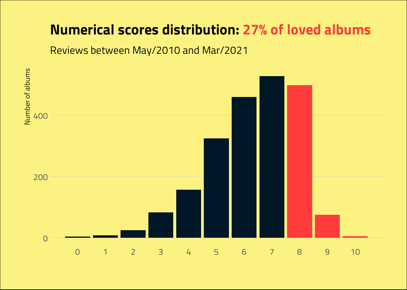
Not every album is blessed with a high score from Melon. The mean score was 6.33, with most of the albums getting a 7.
palette <- c("#fcf281", "#011627", "#ff3b3b", "#AF4D98", "#EFCFE3")

min_date <- paste0(month(min(album_review_features$review_date),
                         label = TRUE,
                         locale = 'English_United States.1252'),
                   "/",
                   year(min(album_review_features$review_date)))

max_date <- paste0(month(max(album_review_features$review_date),
                         label = TRUE,
                         locale = 'English_United States.1252'),
                   "/",
                   year(max(album_review_features$review_date)))
album_review_features %>%
        count(score) %>%
        filter(!is.na(score)) %>%
        ggplot(aes(x = score, y = n)) +
        geom_col(aes(fill = score >= 8), show.legend = FALSE) +
        scale_fill_manual(values = palette[c(2, 3)]) +
        scale_x_continuous(breaks=seq(0, 10)) +
        labs(title = glue("Numerical scores distribution: <span style='color:#ff3b3b'>{round(100 * mean(album_review_features$score >= 8, na.rm = TRUE))}% of loved albums</span>"),
             subtitle = glue("Reviews between {min_date} and {max_date}"),
             y = "Number of albums",
             x = "") +
        theme_ipsum_tw(grid = "Y") +
        theme(
                plot.background = element_rect(fill = palette[1]),
                plot.title = element_markdown()
        )
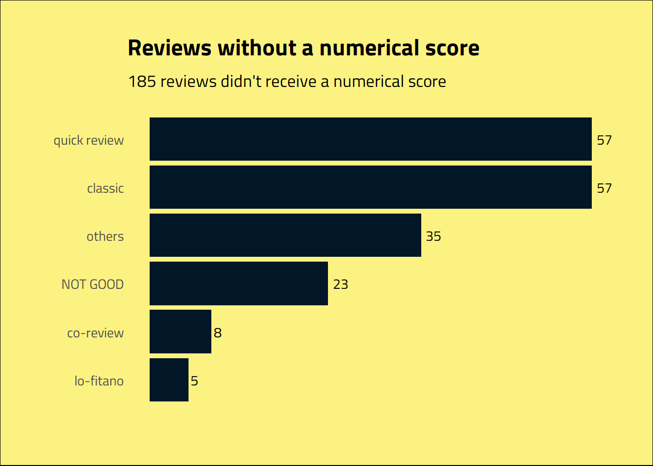
Some of the albums didn’t receive a numeric score. They are summarised in the word_score attribute of our data. As shown below, the classics, quick reviews, NOT GOOD, co-review and lo-fitano fall into this category, as the Cal Chuchesta throwing up on the Lady Gaga’s Born This Way review.

album_review_features %>%
    filter(!is.na(word_score)) %>%
    mutate(word_score =
             fct_lump_min(word_score, 3, other_level = "others")
           ) %>%
    count(word_score, sort = TRUE) %>%
    mutate(word_score =
             fct_reorder(word_score, n),
           ) %>%
    ggplot(aes(x = word_score, y = n, label = n)) +
    geom_col(fill = palette[2]) +
    geom_text(aes(x = word_score, y = n), family = "Titillium Web",
              hjust = -.3) +
    labs(x = "", y = "",
         title = "Reviews without a numerical score",
         subtitle =  glue("{album_review_features %>% filter(!is.na(word_score)) %>% nrow()} reviews didn't receive a numerical score")) +
    coord_flip() +
    theme_ipsum_tw(grid = "") +
    theme(
        plot.background = element_rect(fill = palette[1]),
        axis.text.x = element_blank()
        )
Preparing the Data
Working with genres
We have 358 genres, of which the most common are alternative hip hop, alternative dance, art pop, alternative rock, and hip hop. That is a lot of different categories to work with.

To deal with it, I replaced the specifics subgenres with a more broad view of the genres: instead of “alternative hip hop”, “hip hop”, “atl hip hop” and the variations that appear on the data, let’s just call it “hip hop”. The same idea was applied to rock, metal, punk, pop, folk, r&b, electronic, regional music, experimental, jazz and ambient. Some of the subgenres were too specific (afrofuturism, escape room, chamber psych and permanent wave) and contained too many observations. They were replaced regarding the artists associated with them. Rate Your Music data was a major reference here.
album_review_features %>%
  count(genre, sort = TRUE) %>%
  reactable(highlight = TRUE)
reviews_features_genres <-
album_review_features %>%
rename("subgenre" = genre) %>%
mutate(genre = case_when(
#finding the genres based on the subgenres
str_detect(subgenre, paste(c("hip hop", " rap", "^rap$", " trap", "^trap$",
"boom bap", "^g funk$", "brooklyn drill", "chicago drill", "j-rap",
"soul flow", "urbano espanol", "wu fam"), collapse = "|"))
~ "hip hop",
str_detect(subgenre, paste(c("r&b", "afro psych", "^funk$",
" soul", "^blues$"),
collapse = "|"))
~ "r&b",
str_detect(subgenre, paste(c("pop", "alt z", "boy band", "c86", "j-idol",
"auteur-compositeur-interprete quebecois",
"swedish singer-songwriter",
"irish singer-songwriter"), collapse = "|"))
~ "pop",
str_detect(subgenre, paste(c("metal", "sludge", "black", "deathgrind",
"deathcore", "crossover thrash", "gaian doom", "new wave of osdm"), collapse = "|"))
~ "metal",
str_detect(subgenre, paste(c("rock", "garage psych", "neo-psychedelic", " indie",
"bubblegrunge", "gaze", "grave wave", "austindie",
"australian psych"), collapse = "|"))
~ "rock",
str_detect(subgenre, paste(c("folk", "stomp and holler",
"canadian singer-songwriter"), collapse = "|"))
~ "folk",
str_detect(subgenre, paste(c("punk", "hardcore", " emo", "^emo$",
"grindcore", "mathcore", "screamo", "dreamo"), collapse = "|"))
~ "punk",
str_detect(subgenre, paste(c("jazz", "adult standards"), collapse = "|")) ~ "jazz",
str_detect(subgenre, paste(c("chillwave", "bass music", "downtempo", "electronica",
"^ai$", "abstract", "australian dance", "^future funk$",
"ambient techno", "house", "bass", "elect", "grime",
"wonky", "brostep", "club",
"big beat", "chillhop", "balearic",
"bmore", "breakcore", "complextro", "edm", "footwork",
"hardvapour", "horror synth"), collapse = "|"))
~ "electronic",
str_detect(subgenre, paste(c(" country", "latin",
"alternative americana", "afrobeat", "chicha"), collapse = "|"))
~ "regional music",
str_detect(subgenre, paste(c("industrial", "drone", "experimental",
"plunderphonics", "laboratorio"), collapse = "|")) ~
"experimental",
str_detect(subgenre, paste(c("hauntology", " ambient"), collapse = "|")) ~
"ambient",
#hardcoding genres of the subgenre afrofuturism
str_detect(artist, paste(c("Africa Hitech", "Flying Lotus"), collapse = "|")) ~ "electronic",
str_detect(artist, paste(c("Alice Coltrane", "Kamasi Washington",
"Matana Roberts", "Sons of Kemet"), collapse = "|")) ~ "jazz",
str_detect(artist, "^FKA") ~ "pop",
str_detect(artist, paste(c("Moor Mother", "Shabazz Palaces"), collapse = "|")) ~ "hip hop",
str_detect(artist, paste(c("Janelle Monáe", "Kelela", "Kevin Abstract",
"Solange", "Steve Lacy", "THEESatisfaction",
"Thundercat", "Willow Smith"), collapse = "|")) ~ "r&b",
#hardcoding genres of the subgenre escape room
str_detect(artist, paste(c("100 gecs", "Alice Glass", "Clarence Clarity",
"DJ Sabrina the Teenage DJ", "^Salem$",
"Slauson Malone", "^gupi$"), collapse = "|")) ~ "electronic",
str_detect(artist, paste(c("Anderson .Paak", "^Boots$", "ECCO2K",
"^Jai Paul$", "Kaytranada"), collapse = "|")) ~ "r&b",
str_detect(artist, paste(c("Flatbush Zombies", "^Heems$", "^Lil B$",
"Little Simz", "Princess Nokia", "Ratking"), collapse = "|")) ~ "hip hop",
str_detect(artist, "Kero Kero Bonito") ~ "pop",
#hardcoding genres of the subgenre chamber psych
str_detect(artist, paste(c("Fontaines D.C.", "Protomartyr", "^Shame$",
"Sleaford Mods"), collapse = "|")) ~ "punk",
str_detect(artist, "Ghostpoet") ~ "electronic",
#hardcoding genres of the subgenre permanent wave
str_detect(artist, "Green Day") ~ "punk",
str_detect(artist, "Coldplay") ~ "pop",
TRUE ~ subgenre)) %>%
mutate(genre = fct_lump_min(genre, 3, other_level = "not found"))Most of the reviewed albums fall into the hip hop genre, followed by rock, pop, metal, electronic, punk and alternative dance. Goodbye wu fam, plunderphonics and meme rap.
reviews_features_genres %>%
  mutate(genre = as.character(genre),
         genre = case_when(
    is.na(genre)~ "genre or subgenre not found",
    genre == "not found" ~ "genre or subgenre not found",
    TRUE ~ genre)) %>%
  count(genre, sort = T) %>%
  ggplot(aes(x =reorder(genre, n), y = n)) +
  geom_col(aes(fill = (genre == "hip hop"),
               alpha = (genre == "genre or subgenre not found")), show.legend = FALSE) +
  geom_text(aes(label = n,
                alpha = (genre == "genre or subgenre not found"),
                col = (genre == "hip hop")),
            hjust = -.3, show.legend = FALSE,
            family = "Titillium Web Light") +
  scale_alpha_manual(values = c(1, .3)) +
  scale_fill_manual(values = c(palette[2], palette[3])) +
  scale_color_manual(values = c(palette[2], palette[3])) +
  coord_flip() +
  labs(title = "<span style='color:#ff3b3b'>**Hip hop**</span> is the most reviewed genre",
       x = "",
       y = "") +
  ylim(c(0,580)) +
  theme_ipsum_tw(grid = "") +
  theme(
        plot.background = element_rect(fill = palette[1]),
        axis.text.x = element_blank(),
        plot.title = element_markdown())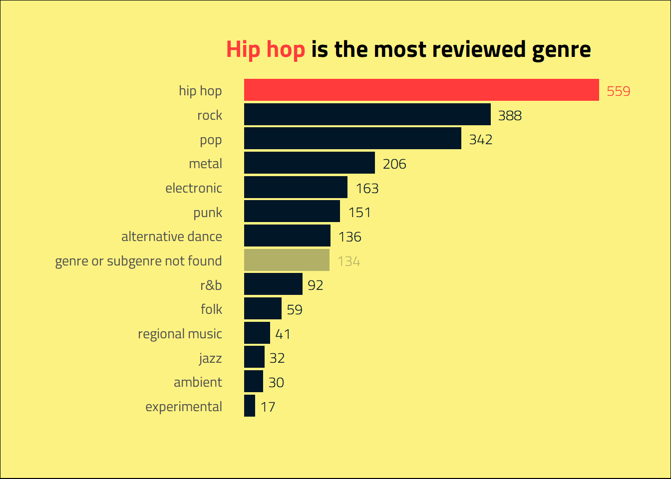
Dealing with missing albums and scores
Albums without numerical scores and the albums that I didn’t find on Spotify weren’t considered. So, filtering that data, we have a total of 2097 albums to create our predictors, target and labels.
na_rm_data <-
  reviews_features_genres %>%
  filter(!is.na(score), !is.na(album_uri)) %>%
  mutate(loved = 1*(score >= 8),
         artist = str_replace(artist,
                              pattern = "Kirin J Callinan",
                              replacement = "Kirin J. Callinan"),
         genre = fct_lump_min(genre, 50, other_level = "others"),
         genre = as.character(genre),
         genre = case_when(
    is.na(genre) & str_detect(artist, paste(c("Wild Flag", "The Debauchees",
                                              "Snake Oil", "Little Women",
                                              "Jesu, Sun Kil Moon", "Guardian Alien",
                                              "Dweller On the Threshold", "Andrew W.K."), collapse = "|"))
    ~ "rock",
    is.na(genre) & str_detect(artist, paste(c("Ty Segall Band", "Soupcans",
                                              "OFF!", "lobsterfight", "Hoax",
                                              "Haunted Horses", "Calvaiire"), collapse = "|"))
    ~ "punk",
    is.na(genre) & str_detect(artist, paste(c("The Log.Os", "Lee Bannon",
                                              "H-SIK", "Evian Christ", "Arca"), collapse = "|"))
    ~ "electronic",
    is.na(genre) & str_detect(artist, paste(c("The Act of Estimating as Worthless",
                                              "Phoebe Bridgers"), collapse = "|"))
    ~ "folk",
    is.na(genre) & str_detect(artist, paste(c("Red Horse", "Otis Brown III", "Okonkolo"), collapse = "|"))
    ~ "others",
    is.na(genre) & str_detect(artist, paste(c("Magic Kids", "Kirin J. Callinan",
                                              "Jonathan Rado", "Hayley Williams"), collapse = "|"))
    ~ "pop",
    is.na(genre) & str_detect(artist, paste(c("Spirit Possession", "Sisu", "Lycus"), collapse = "|"))
    ~ "metal",
    is.na(genre) & str_detect(artist, paste(c("Sisyphus", "Rural Internet",
                                              "Mr. Yote", "Future", "93PUNX, Vic Mensa"), collapse = "|"))
    ~ "hip hop",
    TRUE ~ genre
  ))

predictors <-
  na_rm_data %>%
  select(genre, album_length_min, mean_track_duration:sonic_anger)

target <-
        na_rm_data %>%
        select(loved)

labels <-
        na_rm_data %>%
        select(album_id, album_uri, title, artist, genre, score)
Splitting the data
Let’s go to Python to preprocess the data using Scikit-Learn. First, the data was imported into the Python environment. The train/test splitting was stratifying by the score values, considering that we have few observations with very low (0-3) and very high (9-10) scores.
from sklearn.model_selection import train_test_split

X = r.predictors
y = r.target

X_train, X_test, y_train, y_test = train_test_split(X, y, test_size = 0.2, stratify=y, random_state=42)

y_train_values = y_train.values.ravel() #array of values
y_test_values = y_test.values.ravel()
Scaling and encoding
I preprocessed the train data first to avoid data leakage (see, for instance, the Bex T. post on Towards Data Science). The missing numeric features were imputed with the median values. The categorical features were encoded with One Hot Encoder, and the numerical features were scaled with the standard scaler.
from sklearn.preprocessing import OneHotEncoder
from sklearn.compose import ColumnTransformer
from sklearn.preprocessing import StandardScaler
from sklearn.impute import SimpleImputer
from sklearn.pipeline import Pipeline
import pandas as pd
import numpy as np

X_train = X_train.fillna(np.nan)

num_attribs = list(X_train.drop(columns = ["genre"]))
cat_attribs = ["genre"]

num_pipeline = Pipeline([
    ("imputer", SimpleImputer(strategy = "median", missing_values=np.nan)),
    ("std_scaler", StandardScaler())
])

cat_pipeline = Pipeline([
    ("one_hot", OneHotEncoder())
])

full_pipeline = ColumnTransformer([
    ("num", num_pipeline, num_attribs),
    ("cat", cat_pipeline, cat_attribs)
])

X_train_prep = full_pipeline.fit_transform(X_train)
Supervised Learning Modeling
The data is quite unbalanced. If we measure our success with accuracy, a dummy model that considers that Fantano didn’t love any album would get a 74% score on train data. But who wants such a sad world with no loved albums? So, I trained a classification model looking for optimizing the total Area Under the Curve (AUC) metric, trying to find a classifier that shows if Melon would love an album.
Fine I’ll do one pic.twitter.com/LyI25O8FXV
— Chelsea Parlett-Pelleriti (@ChelseaParlett) June 13, 2021
Dummy predictor
As a base estimator, let’s create a classifier that considers that Fantano doesn’t love any album, which results in an AUC score of 0.5. Our goal is to find something better than that.
from sklearn.metrics import confusion_matrix
from sklearn.metrics import roc_auc_score
from sklearn.metrics import roc_curve
from sklearn.dummy import DummyClassifier

dummy_clf = DummyClassifier(strategy="most_frequent")
dummy_clf.fit(X_train_prep, y_train_values)
## DummyClassifier(strategy='most_frequent')dummy_pred = dummy_clf.predict(X_train)
dummy_roc_auc = roc_auc_score(y_train_values, dummy_pred)
confusion_matrix(y_train_values, dummy_pred)## array([[1237, 0],
## [ 440, 0]], dtype=int64)Random Forest
Due to the considerable number of predictors and complexity of the task, I focused on ensemble learning algorithms. I started with a Random Forest Classifier - the popular ensemble of Decisions Trees. For hyperparameter tuning, I applied RandomSearchCV, tunning the minimum number of samples in each node before splitting (min_samples_split), the minimum number of samples in each leaf (min_samples_leaf) and the maximum number of features evaluated for each splitting (max_features). The ranges of values for tunning the parameters were selected after running the randomized search a couple of times.
from sklearn.ensemble import RandomForestClassifier
from sklearn.model_selection import RandomizedSearchCV

rf_clf = RandomForestClassifier(random_state = 42, n_estimators=500)
rf_params = {"min_samples_split": np.linspace(2, 30, num = 29).astype(int),
            "min_samples_leaf": np.linspace(1, 10, num = 10).astype(int),
            "max_features": ["log2", "sqrt"]}

rf_rscv = RandomizedSearchCV(rf_clf, rf_params, cv=3,return_train_score=True, scoring = "roc_auc")
rf_rscv.fit(X_train_prep, y_train_values)
## RandomizedSearchCV(cv=3,
## estimator=RandomForestClassifier(n_estimators=500,
## random_state=42),
## param_distributions={'max_features': ['log2', 'sqrt'],
## 'min_samples_leaf': array([ 1, 2, 3, 4, 5, 6, 7, 8, 9, 10]),
## 'min_samples_split': array([ 2, 3, 4, 5, 6, 7, 8, 9, 10, 11, 12, 13, 14, 15, 16, 17, 18,
## 19, 20, 21, 22, 23, 24, 25, 26, 27, 28, 29, 30])},
## return_train_score=True, scoring='roc_auc')rfc = rf_rscv.best_estimator_We can see that precision falls quickly. It is far from the perfect classifier, but it shows some improvement compared to the baseline classifier. With a threshold of 0.2, we get close to 80% of the loved albums with precision near 30%. With a threshold of 0.5, almost no loved album would be identified.
from sklearn.model_selection import cross_val_predict
from sklearn.metrics import precision_recall_curve
import matplotlib
import matplotlib.pyplot as plt

def plot_rec_prec(trained_model, plot_title):
  y_scores = cross_val_predict(trained_model, X_train_prep, y_train_values, cv = 3, method = "predict_proba")
  precisions, recalls, thresholds = precision_recall_curve(y_train_values, y_scores[:,1])

  plt.subplot(1, 2, 1)
  plt.plot(recalls, precisions)
  plt.grid(True)
  plt.xlabel("Recall")
  plt.ylabel("Precision")
  plt.title(plot_title)
  plt.xticks(np.arange(0, 1.01, step=0.1))
  plt.yticks(np.arange(0, 1.01, step=0.1))

  plt.subplot(1, 2, 2)
  plt.grid(True)
  plt.plot(thresholds, precisions[:-1], "b--", label = "Precision")
  plt.plot(thresholds, recalls[:-1], "g-", label ="Recall")
  plt.xlabel("Threshold")
  plt.yticks(np.arange(0, 1.01, step=0.1))
  plt.legend()
plt.close()
plot_rec_prec(rfc, "Random Forest: precision and recall")
plt.show()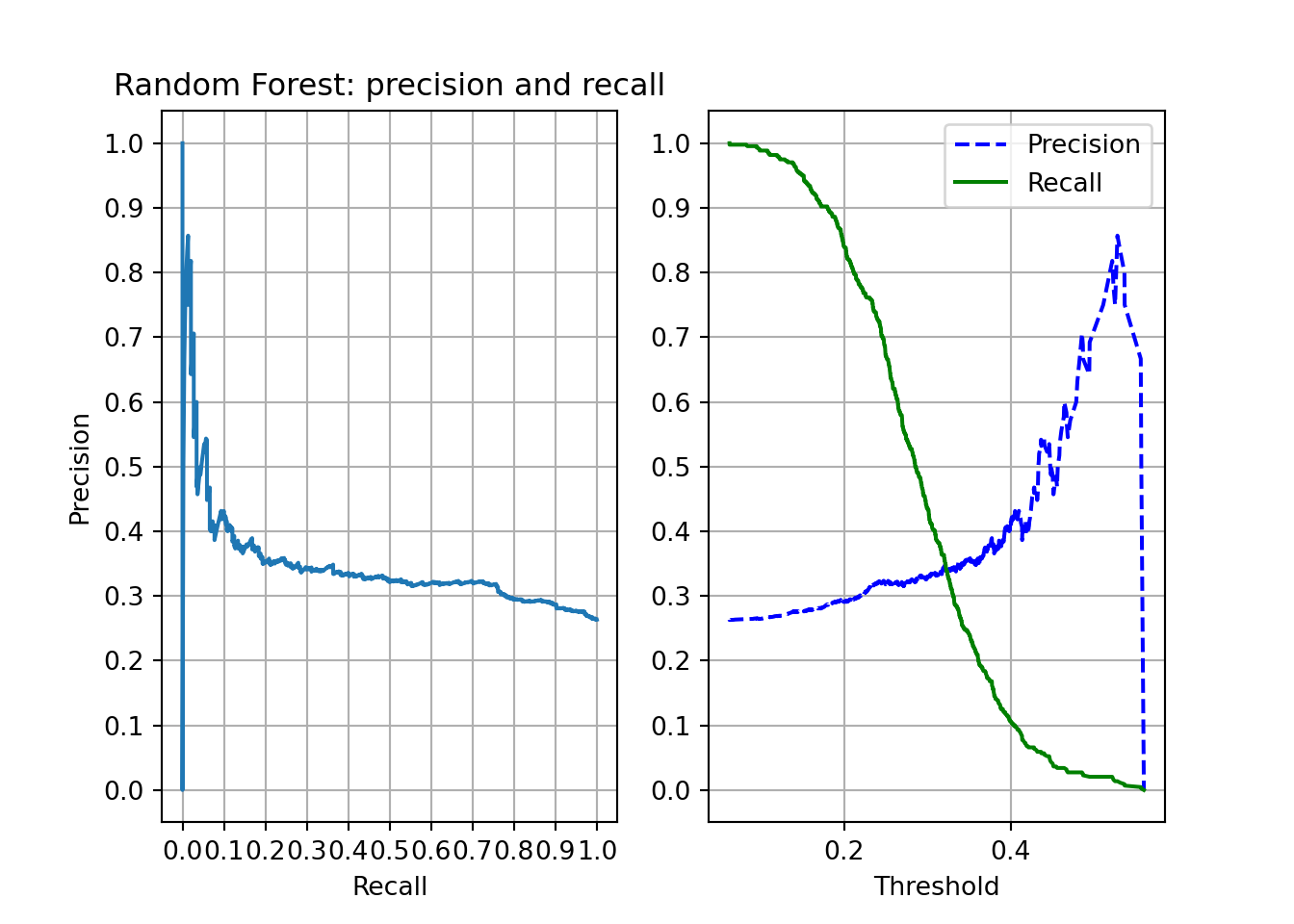
from sklearn.model_selection import cross_val_score

rf_scores = cross_val_score(rfc, X_train_prep, y_train_values, scoring = "roc_auc", cv=10)
Extremely Randomized Trees
The Extremely Randomized Trees (or Extra-trees) model makes the Random Forest more random by using random thresholds for each feature. I thought about giving it a try, checking if a higher randomization level could improve the results. I also performed hyperparameter tunning in min_samples_split, min_samples_leaf and max_features.
from sklearn.ensemble import ExtraTreesClassifier

et_clf = ExtraTreesClassifier(random_state = 42, n_estimators=500)

et_params = [
    {"min_samples_split": np.linspace(2, 30, num=29).astype(int),
    "min_samples_leaf": np.linspace(1, 10, num = 10).astype(int),
    "max_features": ["log2", "sqrt"]}]

et_rscv = RandomizedSearchCV(et_clf, et_params, cv=3, return_train_score=True, scoring = "roc_auc")
et_rscv.fit(X_train_prep, y_train_values)
## RandomizedSearchCV(cv=3,
## estimator=ExtraTreesClassifier(n_estimators=500,
## random_state=42),
## param_distributions=[{'max_features': ['log2', 'sqrt'],
## 'min_samples_leaf': array([ 1, 2, 3, 4, 5, 6, 7, 8, 9, 10]),
## 'min_samples_split': array([ 2, 3, 4, 5, 6, 7, 8, 9, 10, 11, 12, 13, 14, 15, 16, 17, 18,
## 19, 20, 21, 22, 23, 24, 25, 26, 27, 28, 29, 30])}],
## return_train_score=True, scoring='roc_auc')etc = et_rscv.best_estimator_The precision and recall plots are pretty like the ones on Random Forest, although the results seem slightly better – i.e., for a threshold of 0.2, we got a recall near .85.
plt.close()
plot_rec_prec(etc, "Extra-Tree: precision and recall")
plt.show()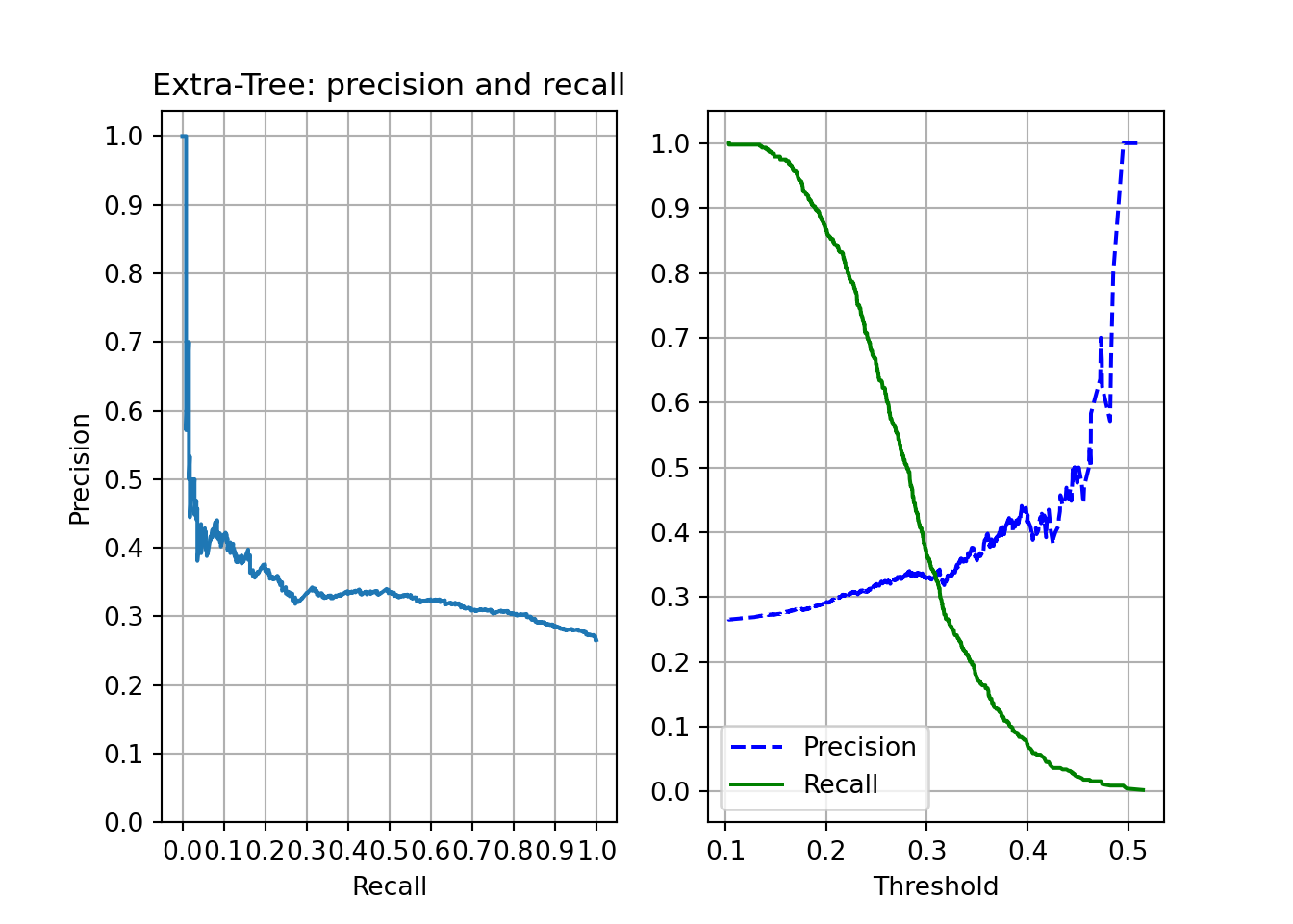
et_scores = cross_val_score(etc, X_train_prep, y_train_values, scoring="roc_auc",cv=10)Logistic Regression
This is the simplest model to use and interpret in this post. I fitted a logistic regression model using a ridge regularization (setting penalty = “l2”), and tunned the inverse of regularization strength (C) hyperparameter.
from sklearn.linear_model import LogisticRegression

logit_clf= LogisticRegression(random_state=42, penalty="l2", solver="liblinear")

logit_costs = [{"C": np.geomspace(1e-4, 1e1, 20)}]

logit = RandomizedSearchCV(logit_clf, logit_costs, cv=3, return_train_score=True, scoring = "roc_auc")

logit.fit(X_train_prep, y_train_values)
## RandomizedSearchCV(cv=3,
## estimator=LogisticRegression(random_state=42,
## solver='liblinear'),
## param_distributions=[{'C': array([1.00000000e-04, 1.83298071e-04, 3.35981829e-04, 6.15848211e-04,
## 1.12883789e-03, 2.06913808e-03, 3.79269019e-03, 6.95192796e-03,
## 1.27427499e-02, 2.33572147e-02, 4.28133240e-02, 7.84759970e-02,
## 1.43844989e-01, 2.63665090e-01, 4.83293024e-01, 8.85866790e-01,
## 1.62377674e+00, 2.97635144e+00, 5.45559478e+00, 1.00000000e+01])}],
## return_train_score=True, scoring='roc_auc')logit_best = logit.best_estimator_The precision-recall plots are not like the previous ones. With high thresholds (>0.8), none album is identified as loved. Also, the precision-recall curve show some bouncing near recall = 0. The results seem slightly worse than the ensemble models.
plt.close()

plot_rec_prec(logit_best, "Logistic Regression: precision and recall")
plt.show()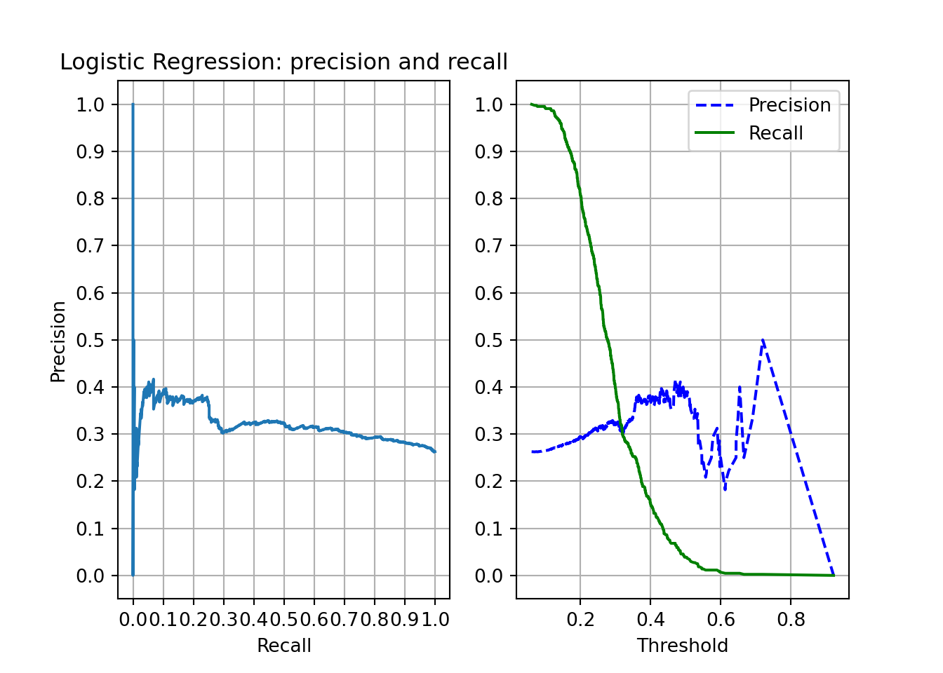
log_reg_scores = cross_val_score(logit_best, X_train_prep, y_train_values, scoring="roc_auc", cv=10)Comparing the models
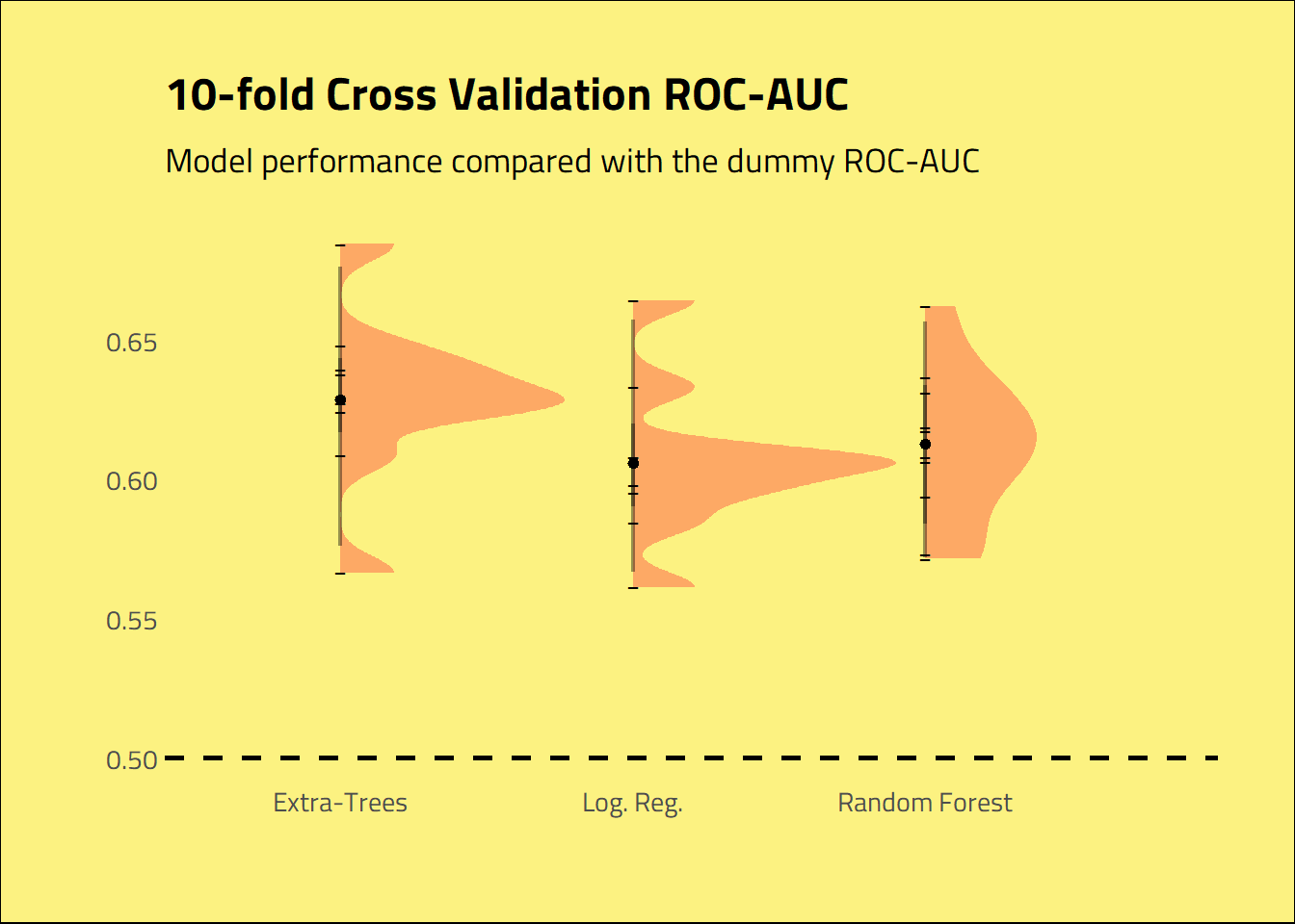
The models beat the dummy regressor, but not by an enormous difference. Extra-trees and random forest seem to outperform the logistic regression model. It looks like the extra-tree model got an AUC score slightly greater than the Random Forest.
modeling_roc_auc <-
    tibble(
           extra_tree = py$et_scores,
           random_forest = py$rf_scores,
           log_reg = py$log_reg_scores) %>%
    pivot_longer(cols = c("extra_tree", "random_forest", "log_reg")) %>%
    mutate(name = as.factor(name),
           name = fct_recode(name,
               "Extra-Trees" = "extra_tree",
               "Random Forest" = "random_forest",
               "Log. Reg." = "log_reg"
           ))  %>%
    rename(Model = name)

modeling_roc_auc %>%
    ggplot(aes(x = Model, y = value)) +
    stat_halfeye(alpha = 0.4, fill=palette[3], point_alpha = 1, size = 2) +
    geom_point(shape=95, size = 2) +
    geom_hline(yintercept =  py$dummy_roc_auc, size = 1, lty = 2) +
    labs(title = "10-fold Cross Validation ROC-AUC",
         subtitle = "Model performance compared with the dummy ROC-AUC",
         y = "",
         x = "") +
        theme_ipsum_tw(grid = "") +
        theme(
                plot.background = element_rect(fill = palette[1])
        )
Predicting and evaluating the data
With the trained model, we can try to predict if an album is loved by Fantano. I transformed the test data using the full pipeline used in the training data, predicted the probability of an album being loved, and calculated the AUC score.
#preprocess the test data
X_test_prep = full_pipeline.transform(X_test)
#predict the probability of the album get a high score with the Extra-tree model
y_pred_proba = etc.predict_proba(X_test_prep)
#AUC score
test_roc_auc = roc_auc_score(y_test_values, y_pred_proba[:, 1])
#False positive rate, true positive rate and thresholds
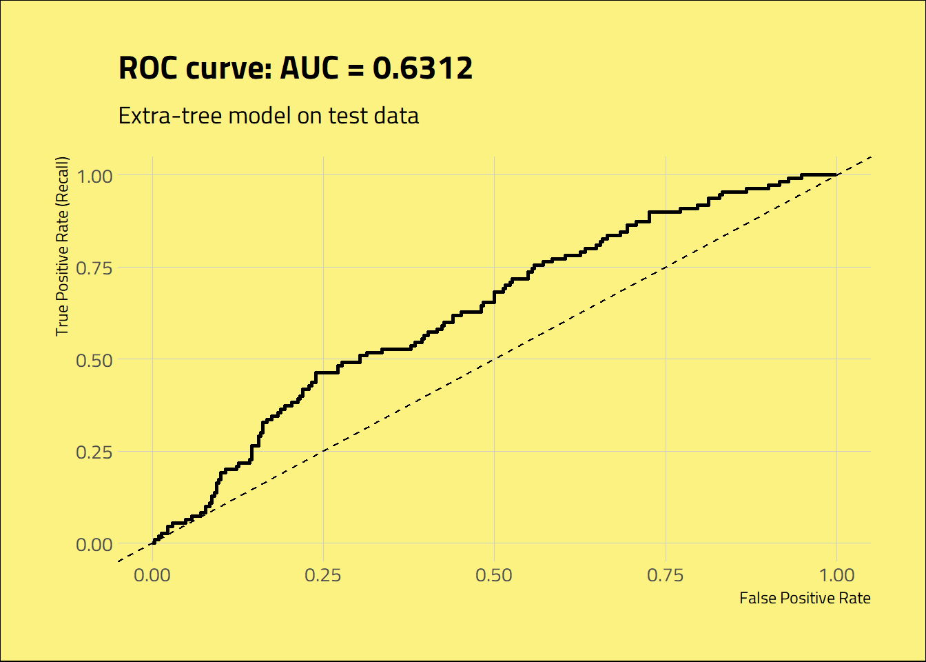
fpr, tpr, thresholds = roc_curve(y_test_values, y_pred_proba[:,1])The selected model achieved an AUC score of 0.6312, better than the dummy predictor and similar to the value found on the train set with cross-validation. It’s a quite limited classifier, but it can help distinguish the loved albums to some extent.
tibble(fpr = py$fpr, tpr = py$tpr, thresholds = py$thresholds) %>%
  ggplot(aes(x = fpr, y = tpr)) +
  geom_line(size = 1) +
  geom_abline(slope = 1, lty = 2) +
  labs(title = glue("ROC curve: AUC = {round(py$test_roc_auc, 4)}"),
       subtitle = "Extra-tree model on test data",
       y = "True Positive Rate (Recall)",
       x = "False Positive Rate") +
  theme_ipsum_tw(grid = "XY") +
  theme(
    plot.background = element_rect(fill = palette[1])
        )
cat_encoder = full_pipeline.named_transformers_['cat']
cat_one_hot_attribs = list(cat_encoder['one_hot'].categories_[0])
attributes = num_attribs + cat_one_hot_attribs
The mean danceability of the album, standard deviation of its liveness, the standard deviation of its energy, and mean instrumentalness are the most important features of the model. To evaluate how they influence the data, let’s do a Partial Dependence Plot (PDP).
feat_importance <- tibble(importance = py$etc$feature_importances_,
                          feature = py$attributes) %>%
  arrange(desc(importance))

feat_importance %>%
  ggplot(aes(x = reorder(feature, importance), y =importance )) +
  geom_col(aes(
    fill = (feature %in% (head(feature, 4)))
    ), show.legend = FALSE) +
  scale_fill_manual(values = palette[c(4, 5)]) +
  coord_flip() +
  labs(x = "",
       y = "",
       title = "Feature importance") +
   theme_ipsum_tw(grid = "X") +
   theme(
     plot.background = element_rect(fill = palette[1]))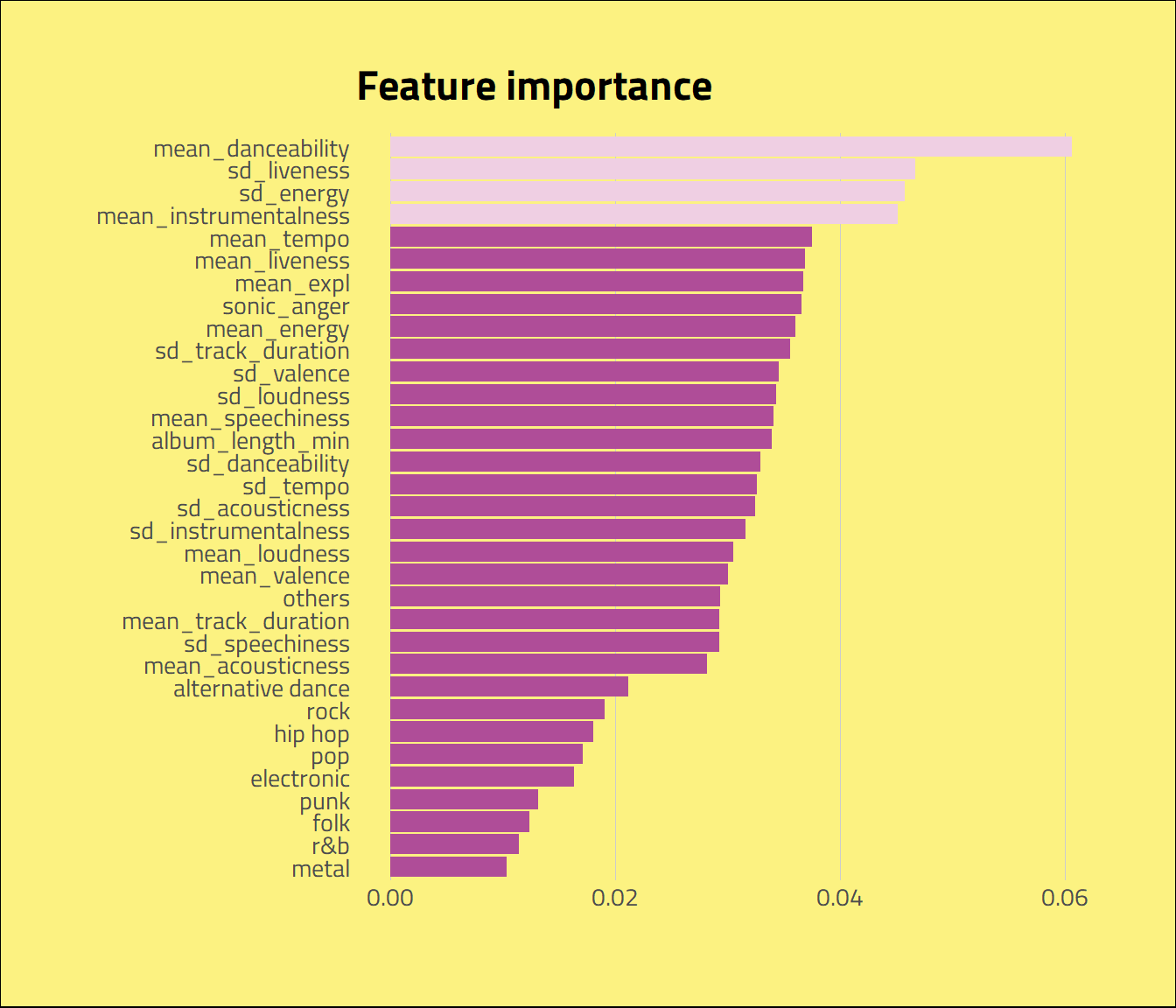
We see that, on average, increasing mean danceability of an album drops the chances of an album being loved. Also, increasing the standard deviation of liveness, the standard deviation of energy, and mean instrumentalness increase the chances of Fantano loving an album.
from sklearn.inspection import plot_partial_dependence

train_prep_df = pd.DataFrame(X_train_prep)

train_prep_df.columns = attributes

plt.close()
display = plot_partial_dependence(etc, train_prep_df, features = ['mean_danceability', 'sd_liveness', 'sd_energy', 'mean_instrumentalness'])
display.figure_.subplots_adjust(wspace=0.4, hspace=0.3)
plt.show(display.figure_)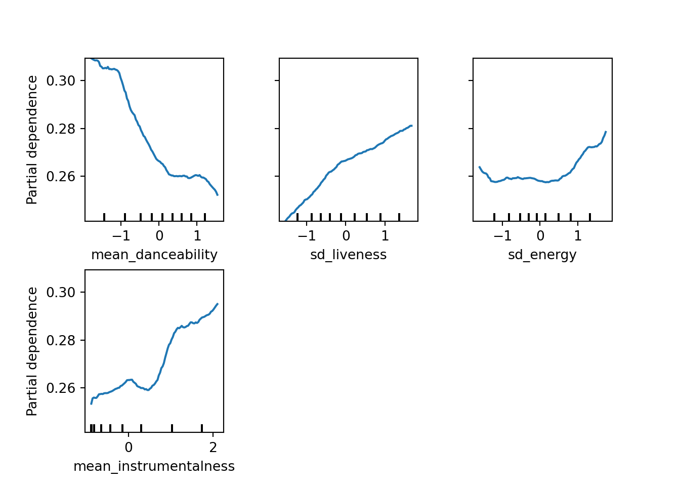
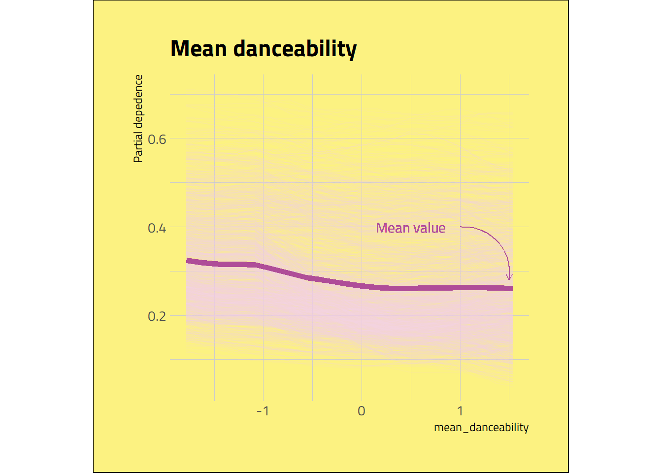
I wanted to check how the mean danceability of an album affected the dependence of the prediction for each instance. So, I plotted the individual conditional expectation (ICE) curve. I couldn’t obtain the ICE curve values with reticulate, so I got it with Jupyter Notebook. The ICE plot shows that mean danceability doesn’t markedly influence the predicted values for some albums with a higher probability of being loved. But, although with some noise, the plot reveals a decreasing predicted chance of getting a high score when increasing the mean danceability.
pdp_individual <- read.csv("./input/pdp.csv")

pdp <-
  tibble(pdp_individual) %>%
  pivot_longer(!val,
               names_to = "sample",
               values_to = "partial")

pdp_mean <- pdp %>%
  group_by(val) %>%
  summarise(partial_mean = mean(partial))

ggplot(data = pdp, mapping = aes(x = val, y = partial)) +
  geom_line(mapping = aes(group = sample), alpha = .1, col = palette[5]) +
  geom_line(data = pdp_mean, mapping = aes(x = val, y = partial_mean), col = palette[4], size = 2) +
  geom_text(aes(x = 0.5, y = 0.4, label = "Mean value"), col = palette[4],
            family = "Titillium Web") +
  geom_curve(aes(x = 1, xend = 1.5, y = 0.4, yend = 0.28),
             arrow = arrow(length = unit(0.07, "inch")), size = 0.4,
             curvature = -0.5, col = palette[4]) +
  labs(title = "Mean danceability",
       x = "mean_danceability",
       y = "Partial depedence") +
  coord_fixed(ratio = 4.5) +
  theme_ipsum_tw(grid = "XxYy") +
  theme(
    plot.background = element_rect(fill = palette[1]),
    plot.title = element_markdown()
  )
Conclusion
I fitted a classification model on the Needle Drop scores using the Spotify data as predictors. As a real-world model, it is a limited classifier. So, although Anthony will not be replaced by a machine (at least not yet), the data showed some interesting insights about what is going on in Melon’s head. And yeap, Fantano does not like to dance.
tran…SITION
Thanks for reading! I’m open to any feedback or constructive criticism. You can reach me on Twitter @_danielbrito_